PROJECT 4
MUTANT MAPPING WITH MOLECULAR MARKERS
![]()
OBJECTIVES:
A phenotypic mutation isolated in a previous semester will be mapped onto the Arabidopsis genome using CAPS/InDel/SSLP molecular markers.
BACKGROUND:
Producing a map of where genes lie within the genome provides an idea of genome organization, evolution of gene families and provides a basis for genome sequencing. The map uses two types of markers: phenotypic markers, relating to an observable mutation of a gene, and molecular markers, relating to a known DNA sequence polymorphism present at a certain location. Maps have been created for many plants of scientific or economic importance.
Maps are also very useful for forward genetics. Isolating and characterizing phenotypic mutants is a powerful means of dissecting a process in an organism. Genetics alone can provide models for how the mutated gene may interact with other components and can suggest a possible function. However, the cloning of the gene responsible for a certain phenotypic mutation allows a more powerful and detailed analysis of function. Mapping of a new phenotypic mutant onto a genetic map for that organism allows one to clone the gene responsible for that phenotype. In plants that do not have a sequenced genome, genome walking provides a means of going from a molecular marker that maps close to your gene to the gene responsible for the phenotype. For plants such as arabidopsis with sequenced genomes, the mapping of a mutation to a certain location on a specific chromosome allows one to find the gene within the database of chromosomal sequences. This project will map a phenotypic mutation onto the arabidopsis map, using molecular markers already present on the arabidopsis map.
Requirements for mapping:
A distance between two loci on a map is measured in recombination frequency. Recombination occurs either by independent segregation of different chromosomes, or by recombination between homologous chromosomes during meiosis. Consider crossing two homozygous mutants, each mutated in a separate gene. The F1 population is uniformly heterozygous for each mutation. However, when the F1 progeny undergo meiosis to produce gametes, reassortment of homologues chromosomes and recombination (crossing over) between homologous chromosomes occur. Recombination is seen in the F2 generation from the self-pollination of the F1 gametes. If each trait is encoded on separate chromosomes, 50% of the progeny have recombinant traits- one mutant trait from one parent, the other mutant trait from the other parent. If both traits are on the same chromosome, the frequency of recombinant progeny is lower than if they are on different chromosomes. The closer two loci, the lower the chance that a recombination event can occur between the two loci. The farther apart the two loci, the higher the frequency that recombination occurs.
The main idea of mapping is to look at a set of F2 progeny. This set of progeny is called the mapping population. Each progeny is scored for one trait at a time as to whether that trait came from parent A or parent B. When this is compared for two traits, the number of progeny showing the recombinant traits (one from one parent, the other from the other parent) is divided by the total number of progeny scored to produce the recombination frequency. This recombination frequency is the map distance between the genes encoding each trait (1 recombinant in 100 progeny = 1% recombination = 1cM).
Creating a mapping population:
The first step in creating a mapping population is in setting up the first cross so that you can follow polymorphisms at different loci. In phenotypic mapping, one crosses your homozygous mutant plant with another mutant plant and study the frequency of recombinants (double mutant or fully wild-type) in the F2 generation. In this case, you can tell the genetic distance between your mutation and this other characterized mutation. Mapping can be made more efficient by crossing with a plant with multiple known mutations and testing the recombination frequency between yours and each of the other mutations. A multiple mutant used in such cross is shown here: http://seeds.nottingham.ac.uk/Nasc/action.lasso?-database=Seed3.fp3&-layout=web&-op=bw&Picture=yes&-op=bw&Seed%20list%20type=Multiple%20marker%20mapping%20lines&-maxRecords=1&-skipRecords=2&-token.user=11639328&-search&-response=detail/detail_general.lasso&-token.page=0&-token.max=25&-token.response=cart/carthitlist2.lasso
Molecular mapping relies upon a different sort of polymorphism to define loci
than having phenotypic mutations- that of sequence differences between the two
parents. In arabidopsis, two different ecotypes are
used. Naturally-occurring DNA sequence differences between the genomes of two
ecotypes (e.g. Landsberg and
Given that others have already created a genetic map of the differences between
two ecotypes, all you have to do is determine the genetic distance between your
new mutation and these molecular markers to place your gene on the
map. Once you have isolated a mutation in one ecotype (e.g.
The mutation we will use is a trichome-less mutant
that was identified in class last year. Like your mutant screen this year, the
mutation was originally found in
Scoring progeny for phenotypic markers
For the phenotypic marker, we will use the visible phenotype to score each progeny in the mapping population for wild-type or mutant genotypes. This is complicated by the fact that most traits have dominant or recessive alleles; the genotype of heterozygous or homozygous dominant individuals can not be determined without further tests. The recessive allele however will be scorable - all progeny showing the recessive phenotype are homozygous recessive. We will pull out all progeny with the recessive phenotype and determine the genotype of the other locus to identify recombinants.
Since the trichomes appear on the first true leaf, we can score the mutations fairly quickly. You will also observe segregation of the erecta gene from the Landsberg parent in this cross.
Scoring Molecular Markers
For molecular markers, scoring phenotype is easier because many molecular markers are co-dominant. This means that one can score the presence of each allele independent of the other allele. We will use three types of molecular markers- CAPS, SSLP and InDel. All use PCR to amplify a segment of the arabidopsis genome and so only a small amount of DNA is needed from each progeny for this analysis.
CAPS stands for Cleavage of Amplified Polymorphic Sites. PCR primers are designed to amplify a small (<1000 bp) region of the genome. Normally, both ecotypes produce the same size PCR product because the overall sequence is similar in both ecotypes. A sequence polymorphism within this region is determined by the ability of a restriction enzyme to cut within this PCR product- the product from one ecotype is cleaved by a specific restriction enzyme while the product from another ecotype is not cleaved. The CAPS marker is scored by gel electrophoresis of the PCR products after restriction enzyme treatment. The progeny bearing the uncut locus will have a DNA product that is the same size as the original PCR product while progeny bearing the locus from the other parent will produce two smaller DNA products, indicating that the PCR product was cut. Examples of Arabidopsis CAPS markers are shown at http://www.arabidopsis.org/maps/CAPS_Chr1.html . The marker name is shown at the left. The PCR primers used to amplify a region in both ecotypes are shown at the far right. The size corresponds to the size of the PCR product that is produced. The enzymes show what restriction enzyme produces differential cutting of the PCR product; you will see different sizes for Columbia (COL) or Landsberg (LER) ecotypes. These CAPS markers have already been placed on the genetic map, as shown as the chromosome (numbered 1-7) and the map position along that chromosome. You can find these locations by placing the locus name into this map search http://www.arabidopsis.org/cgi-bin/maps/Schrom . How does one design CAPS markers in the first place? One starts with the DNA sequence of a particular region. From this sequence, one can choose the PCR primers to use and the presence of restriction enzyme sites within the region (e.g. At this site http://www.arabidopsis.org/cgi-bin/patmatch/RestrictionMapper.pl ) to be amplified. This PCR amplification and restriction enzyme digestion is then tested in another ecotype. If the DNA around the restriction site is polymorphic in the other ecotype, then one finds no cutting for one of the restriction enzymes and the difference defines it as a CAPS marker. An easier way is if the same locations in two ecotypes are sequenced. Then, one looks for locations where two sequences differ at a restriction site. Then PCR primers are designed to flank that polymorphism. Although this seems backwards- needing to know the DNA sequence before making a marker for the region- it is important to remember that making a marker from a certain sequence then allows one to map that DNA sequence relative to others loci on the map. The sequence used for making the CAPS doesn’t need to be a functional gene or the gene your mutation is in, it is just a specific locus in the genome. Together, these provide a ruler against which you measure your mutation. Thus, one basically chooses random dispersed locations around the genome for molecular markers. In the case of genomes that are not totally sequenced (arabidopsis being unusual), randomly chosen clones from a genomic library can sequenced and used to make CAPS markers.
The second molecular marker is the SSLP, for Short Sequence Length Polymorphism (introduction here: http://genome.salk.edu/SSLP_info/Bell_and_Ecker.html ). This is a locus where a repeat of a short DNA sequence exists. These short repeated sequences are hyper-mutable; the number of repeats often differs between ecotypes due to a chance mistake during DNA replication through the repeat. The SSLP marker consists of two PCR primers chosen to flank each side of the short sequence repeat. In one ecotype, the PCR product will be a certain length, say 110 bp including a repeat 10 copies of a 3 bp repeat. PCR amplification of another ecotype using the same primers may produce a 125 bp product - due to the presence of 15 copies of the same repeat. Like the CAPS markers, the SSLP marker can not be predicted beforehand. The DNA sequence for a certain region is searched for a short sequence repeat and flanking PCR primers are designed from the flanking sequence. The size of the PCR product from these primers is then determined using DNA from other ecotypes. If a polymorphism in PCR product length is seen among ecotypes, then it can be used as an SSLP marker. A SSLP marker we will use is at http://www.arabidopsis.org/servlets/TairObject?id=67&type=marker . Note that the PCR primers used to amplify this region is shown, along with the sizes produced from each ecotype’s DNA at that locus. You can also see its position relative to other molecular markers from that page.
InDel
markers are similar to SSLP markers in that they use PCR to amplify a region
which has a length polymorphisms. However, whereas
SSLP detect changes in the number of repeats in a simple sequence, InDel markers take advantage of larger insertions or deletions
that occur in a region. Identifying InDel markers
usually requires comparing genome sequences from two variants (e.g. arabidopsis ecotypes Lansdberg
and
OVERVIEW:
Mapping 1:
Plant seeds of mapping population
Carefully plant the seeds representing the F2 progeny in soil. Try to assure that the soil is fully wetted and the seeds are well spaced. Perform the cold treatment and these will be allowed to grow over the following weeks.
Read instructions:
Planting seeds
Web resources:
Overview of Recombinant Inbred Lines used to make the map
http://nasc.nott.ac.uk/RI_data/how_to_map.html
Pictures of
ecotypes, including Landsberg and
http://vannocke.user.msu.edu/pages/811%20lab/ecotypes.html
Questions to consider:
-How do the seeds you are planting differ from the parent (F1) plants?
-Considering that all these seeds came off of one parent (F1) plant, is every seed the same as each other? What has occurred in producing these seeds that does this?
Mapping
2: Screen seedlings for phenotypes to select mutants/wt
Look through the plants. You are looking at the loss of trichomes in the true leaves. Identify all mutants with a toothpick or string and number them.
Questions to consider:
-What is the frequency of trichome-less mutants in the progeny? What frequency would you expect from this cross? Does this match the expected frequency?
Web sites:
Chi-squared test descriptions:
http://www.cc.ndsu.nodak.edu/instruct/mcclean/plsc431/mendel/mendel4.htm
http://www.ruf.rice.edu/~bioslabs/tools/stats/chisquare.html
Chi-squared table with more degrees of freedom:
http://www.stat.tamu.edu/~west/applets/chisqdemo.html
Chi-squared calculators:
http://graphpad.com/quickcalcs/chisquared1.cfm
Two and three class chi-squared calculator:
http://www.rhul.ac.uk/Biological-Sciences/Archives/Warren/calc/chisq2.html
http://www.rhul.ac.uk/Biological-Sciences/Archives/Warren/calc/chisq3.html
Mapping 3:
Genomic DNA prep from plants
Perform a DNA miniprep from the mutant plants (homozygous since it it recessive) identified in the previous class.
Read instructions:
Plant genomic DNA miniprep
Questions to consider:
This DNA prep differs from the one done for cloning a gene by PCR in that you are processing more samples. What would you expect to see if some of the DNA from one progeny entered a sample from another progeny (a contaminant is only in the wrong place at the wrong time- one man’s precious sample is another’s contaminant)? Remember, PCR is very sensitive and amplifies the DNA present. How would this alter your results?
Mapping 4:
PCR analysis of DNA using molecular markers
PCR reactions will be performed with the CAPS, SSLP and InDel markers. DNA from the different F2 trichome-mutant progeny will be distributed to each student who will perform the PCR required for an appropriate proportion of these progeny. InDel and SSLP markers just require PCR amplification whereas CAPS markers require a restriction enzyme digestion after amplification.
InDel Markers: positions are in Mb, which can be found on the Arabidopsis genome maps
1F15D2 Chromosome 1, 10.3 Mb
1T26J14 Chromosome 1, 25 Mb
2F7D8 chromosome 2, 9.3 Mb
2T8O18 Chromosome 2, 12.2 Mb
3MIE1 Chromosome 3, 4.9 Mb
3MDJ14 chromosome 3, 9.9 Mb
3T21J18 Chromosome 3, 18 Mb
4T4C9 Chromosome 4, 7.3 Mb
4T13J8 Chromosome 4 13.9 Mb
5MYJ24 Chromosome 5, 7.8 Mb
5MUL8 Chromosome 5, 15.7 Mb
CAPS marker SUP 5’-GATCTATGGAGATGACACAAG
5’-GTCAAGATATGGCTCACGAGGA
CAPS marker AFC1 5’-AGCTTTATCACGATACACACTGC
5’-GGAACTCTCAAGTCTAAACAG
cuts with PvuII
CAPS marker M235 5’-AGTCCACAACAATTGCAGCC
5’-GAATCTGTTTCGCCTAACGC
cuts with HinDIII
SSLP marker k7M2F 629 5’-CTCCGCCATATATAATCAGAGAA
5’-GGTTGGTGTTTTCCTCCATT
note- this is from a BAC clone on the map- either search for the BAC clone, or search for one of the sequences to see on the map.
SSLP marker CIW11 5’-CCCCGAGTTGAGGTATT
5’-GAAGAAATTCCTAAAGCATTC
SSLP marker CIW4 5’-GTTCATTAAACTTGCGTGTGT
5’-TACGGTCAGATTGAGTGATTC
Read instructions:
PCR reactions for CAPS , InDel and SSLP markers
Web sites:
CAPSmarkers from Arabidopsis:
http://ausubellab.mgh.harvard.edu/resources/molecular/caps/index.html
Papers describing CAPS markers in Arabidopsis http://www.blackwell-synergy.com/doi/abs/10.1046/j.1365-313X.1993.04020403.x
http://pubs.nrc-cnrc.gc.ca/ispmb/ispmb19/R01-027.pdf
Overview of Molecular Markers:
http://www.cnrs-gif.fr/isv/EMBO/manuals/ch2.pdf
Good description of SSLP markers:
http://carnegiedpb.stanford.edu/publications/methods/ppsuppl/Supplemental1.pdf
Practical description of CAPS markers:
http://www.plantae.lu.se/fskolan/arabidopsistexter/MariaEriksson.html
Questions to consider:
-What
are the DNA sequence polymorphisms that each marker is measuring? Find your
marker on the genetic map (http://www.arabidopsis.org/servlets/mapper)
and find the corresponding location on the sequence map. The map is
-Are these primers going to find a unique segment of the DNA genome. Calculate the frequency of this sequence occurring by the formula
frequency (1 occurrence in the resulting number of base pairs)
= (number of possible bases) length of sequence
for an 18 bp oligonucleotide
frequency = (4)18
Is this sufficient to allow the primer to find a unique site in the genome given Arabidopsis genome size of 1.2 x 10⁸ bp?
-Try the test in silico on the arabidopsis genome- search for the number and location of the CAPS marker m235 primer AGTCCACAACAATTGCAGCC. Click here for searching arabidopsis genome http://mips.gsf.de/proj/thal/db/search/search_frame.html . Remember to choose a nucleotide search. It is on chromosome 1.
Lab
26
Mapping 5: Gel electrophoresis of PCR reactions
The PCR reactions from last time will be analyzed by agarose gel electrophoresis. Due to the smaller size of SSLP markers (due to having to determine smaller differences in repeat lengths), these will be run on a 3 % agarose gel. The CAPS marker PCR products are larger, so they will be run on a 0.8 % agarose gel. The InDel markers are an intermediate size (600-1200 bases) and are run on a 1.4% agarose gel.
Read instructions:
Gel Electrophoresis
Web sites:
Artifacts and problems with CAPS and SSLPs:
http://www.rhul.ac.uk/Biological-Sciences/Archives/Warren/caps.html
Questions to consider:
-For
your marker, which progeny had DNA at that locus that was homozygous
-Are there any uncertainties in your interpretation?
Lab 27 Mapping
6: Database analysis of mapping data
The map distances will be determined by comparing recombination frequencies between the mutant and each of the molecular markers for each progeny. This requires everyone to pool the data on separate markers and progeny.
Read instructions:
Linkage calculations
Finding Map Positions
Web sites:
Determine the position of the markers we are using (click on map on result):
http://www.arabidopsis.org/search/marker_search.html
Discussion of map distances, two and three-point crosses:
http://www.arbor.edu/~michaelb/genmap1.htm
Genome map needed for question below:
http://www.arabidopsis.org/servlets/mapper
Questions to consider:
Which markers are unlinked to the trichome-less gene? Can we say initially which chromosome the mutation is on? Use Chi-squared tests to determine if the observed frequency is significantly different than 50%, which would be unlinked.
Which markers are linked to the trichome-less gene?
How close are these in centimorgans?
By comparing the cM distances and base pair distances on the Arabidopsis map, could you find a general portion of DNA that may contain the gene that determines trichome development? How accurate is this assignment? Would it be to the gene level, lambda clone or BAC clone level of accuracy? How many genes, cosmids or BACs are within the region you mapped the mutation to? Is there any obvious gene in this region that might already be known for trichome development (being a phenotypic trait, look at the markers on the genetic map).
-Also try mapping the molecular markers against each other. Does the genetic distance between them agree with the published map position? In doing this, consider the difficulty of assigning recombinant vs parental labels to progeny that are heterozygous for both molecular markers. Also, in comparing this to the published map, consider that we threw out all plants that were homozygous or heterozygous for the trichome+ wild-type allele. How does this skew the results?
DETAILED PROCEDURES:
Planting mutagenized seed in
soilless mix
1. Scoop the sterilized potting mix (“soil”- but there is no soil, just a mix of peat moss and vermiculite) into 9 white plant pots. The soilless mix has been autoclaved to avoid insect contamination. Try to get the soilless mix even with the top and smooth the surface of the planting mix. Place the filled pots in the green or black trays.
2. Wet the planting mix. First add 2 liters of tap water to the tray. Second, to help the planting mix pick up water and to wet the top layer, use the mister to spray the surface of the planting mix to soak it. Do this before sprinkling on the seed.
3. Plant the seeds. Arabidopis seeds are tiny. For the molecular mapping, the number of seeds are limited- try to make each seed count. Plant 5 seeds per pot, well spaced within the pot. Do not try to cover the seeds with soil, they will germinate best on the surface and touching the soil will probably stick the seeds to your hands.
4. Cover the trays with Saran wrap. The seeds and soil need to be fully hydrated and covering the entire pot will help the water wick up to the top and prevent drying by evaporation. Rip off a piece of Saran wrap the size of the tray and place it over the tray. Tape down the edges.
5. If the seeds were not pre-chilled, provide a cold-treatment. Breaking the dormancy of the seeds requires a 2-3 day cold treatment. Place the planted trays in the cold room (4oC, 40oF). After 2-3 days, carry out and place under the fluorescent lights. Leave the Saran wrap on the trays. Take off the Saran wrap when the first true leaves appear on the seedlings. This will take about 1 week after taking the tray out of the cold room.
Genomic DNA miniprep
1. Add 400 ml Edward extraction buffer to a 1.5 ml eppendorf tube,
2. Take 2-3 small (or 1 large) leaves from one plant using a sharp forceps. Clean the forceps for each plant using a kimwipe.
3. grind the tissue in the eppendorf tube with a pestle that fits the tube. (One pestle/sample).
4. vortex 5 sec, set at room-temperature until all the samples are ready,
5. spin at 14,000 rpm. in a microcentrifuge for 2 min,
6. transfer 350 mls of the supernatant to a fresh tube,
7. Add 350 mls of isopropanol to each tube, mix ,
8. set at room-temperature for 2 min,
9. spin 5 min at 14000 rpm,
10. decant the supernatant, the pellet contains DNA.
11. Add 300 ul of 70% ethanol to each tube to wash the DNA pellet,
12. spin at 14000 rpm for 3 min,
13. decant the supernatant,
14. air dry samples for 30 min by placing the tubes upside-down on a piece of Kimwipe paper
15. re-suspend the DNA pellet in 100 ml distilled water. (This makes 10x DNA template)
16. use 2-5 ml template for PCR
Edward Buffer:
200 mM Tris pH 7.5; 250 mM NaCl,; 25 mM EDTA; 0.5% SDS.
PCR reaction:
Standard conditions for PCR are:
100 nanograms genomic DNA
40 picomoles of each primer
100 mM dNTPs (ATP, CTP, GTP and TTP)
2.5 mM MgCl2 (can vary from 1.5 to 3 mM)
1X Taq polymerase buffer- Tris, detergent, KCl
2 units of Taq polymerase
volume of 50 ml
PCR cycles: 44 cycles of 94oC (denaturing temp.) 30 sec., annealing temperature (determined for primer 56oC for most, 58 or 60 for InDel) for 30 sec., 72oC (extension temp) for 1 min.
There are a couple modifications we will make to this basic procedure:
a) Since only one gel lane is needed for each reaction, we will scale them down to half the volume.
b) To handle the multiple samples efficiently, we will make pools of common components. First, we will make a master mix of the polymerase, dNTP and buffer. We will aliquot this into tubes containing the different primer pairs. Students will work in pairs, using one of these primer-pair mixes to put together PCR reactions with each of the F2 progeny DNA preps.
So:
1. In each tube: add
18 mls primer mix- has 20 pmoles of each primer, taq polymerase,dNTPs,
and buffer
2 mls DNA from leaf prep
2. Add 50-100 mls of light mineral oil to the tube. This will float on top and prevent evaporation of the small volume of solution.
3. Program the PCR machine- the program will be supplied for the different primers assigned. The annealing temperature depends on the primers used (often 56 for SSLP and CAPS), and the extension times at 72oC depend upon the sequence between the primers.
4. place in the PCR machine and set for the appropriate temperature cycles (discussed in class).
5. The PCR reaction will be held at 5oC when it has stopped 3-4 hours later.
For CAPS markers, the PCR reactions will be added to the appropriate restriction enzyme buffer and digeted with 1 unit of that enzyme and digested at 37oC for 3 hours.
M235- digests with HinDIII, AFCI will be digested with PvuII,, SUP will be digested with NruI
Gel Electrophoresis:
1. The agarose gels will be already formed. These are made by melting agarose in electrophoresis buffer (Tris-acetate buffer with EDTA), pouring in the electrophoresis tray, and allowing it to cool. Ethidium bromide is added to the agar in the molten state when is sufficiently cooled. This dye will fluoresce under UV light when it is intercalated into DNA. This allows us to visualize the DNA. Because ethidium bromide is a mutagen, you will wear gloves when handling the gel.
2. Take the PCR reaction tube from the last lab and use a pipettman to remove 20 ml of the PCR reaction (bottom layer- the top is the mineral oil) and place it in a new tube.
3. Add 2 mls of loading dye – this is 60% sucrose with a blue dye- Bromophenol blue- that will act as an electrophoresis marker. The sucrose will make the solution sink.
4. Load the sample-dye mix carefully into one well of the gel. A size marker will be loaded and other group’s samples will be loaded as well.
5. Once all samples are loaded, attach the leads to the power supply- DNA has a negative charge, so it will move from the negative electrode (black - top) to the positive electrode (red - bottom). Turn the voltage to 100 volts.
6. When the bromophenol blue has moved about 12 cm, turn off the power supply and bring the tray to the UV light box (room around the corner in the hall). The TA will help you visualize the gel and get a picture. Be sure to handle the gel only with gloves.
Linkage Calculations
Since the trichome mutation was originally in
Distance (cM) = (2 x # Landsberg homozygous) + (Landsberg/Columbia heterozygous)
2 x total # of progeny
Pool the linkage information with the groups that used other markers. Compare this to the genetic map of arabidopsis.
The uncertainty of the map distance (due to the number of plants sampled and the number of recombinants) with can be estimated by Chi-squared analysis. Plug in the fraction of recombinant as class A and parental (total minus recombinant) as class B. Choose a level of statistical confidence (90%, or 0.1, is fine). The program will return the limits for the frequency, within the confidence limits.
Chi-squared test descriptions:
http://www.cc.ndsu.nodak.edu/instruct/mcclean/plsc431/mendel/mendel4.htm
http://www.ruf.rice.edu/~bioslabs/tools/stats/chisquare.html
Chi-squared table with more degrees of freedom:
http://www.stat.tamu.edu/~west/applets/chisqdemo.html
Chi-squared calculators:
http://graphpad.com/quickcalcs/chisquared1.cfm
Two and three class chi-squared calculator:
http://www.rhul.ac.uk/Biological-Sciences/Archives/Warren/calc/chisq2.html
http://www.rhul.ac.uk/Biological-Sciences/Archives/Warren/calc/chisq3.html
The formula we use assumes that there is a single cross-over event between the trichome mutant and our marker in any recombinant. However, more than one cross-over may occur, especially over longer distances, that would make a recombinant look like a parental type. This tends to underestimate recombination frequencies. More complex mapping functions can be used to account for double crossovers. See the calculator at:
http://www1.rhbnc.ac.uk/biological-sciences/warren/calc/mapfunc.html
Finding
map positions
Go to www.arabidopsis.org
There are two types of maps on this site. Both are found under tools. MAPVIEWER integrates both the genetic map
(units in cM) and a physical map (units in Mbp). SEQUVIEWER
is only the physical map, but integrates the information from the annotation of
the Arabidopsis genome to show predicted genes, cosmids,
transcripts and other information. Since
we are mapping, and all of our data is in genetic linkage, we will need to
enter the genome through centimorgan units in the Mapviewer.
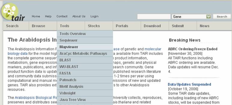
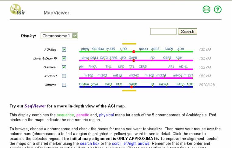
Go to MAPVIEWER. The view of chromosome 1 is the default screen. The different chromosomes shown are different types of maps for chromosome 1. If you are looking for markers or positions on another chromosome, you can select that chromosome from the Display chromosome pull-down bar at the top left. If you are searching for a marker or genetic locus, you can type it into the search box and it will find that marker on any of the chromosomes.
Click here to return to the main menu to see the SEQUVIEWER
Lets say that you were looking for a
region on chromosome 1. The screenshot
above shows different maps you could display in parallel. The AGI (physical),
Lister &Dean RI (genetic) and Classical (genetic) maps are most useful.
Other maps differ with chromosome. The Kazusa map
(physical) is useful on chromosomes 3 and 5. Check on at least the three default maps. To
see a map of a region, click on a part of any of the chromosome map displayed- the exact location you
click is not important since you can move back and forth on the map itself. For
example, clicking at about 1/2 of the distance on chromosome 1 displays the following:

Cosmids in the physical map Markers on the physical map Search for markers here, but always check if the
multiple maps are aligned. You can search for a common marker appearing on
different maps to more accurately align the two maps. Use
these to move the multiple maps back or forth. This will keep
approximate alignment. The Left or
Right buttons on each map will only move that one map and leave the others
unchanged. You can see the rough
alignment in relative positions of the red boxes on the chromosome at the far
left of each map .
![]()


![]()

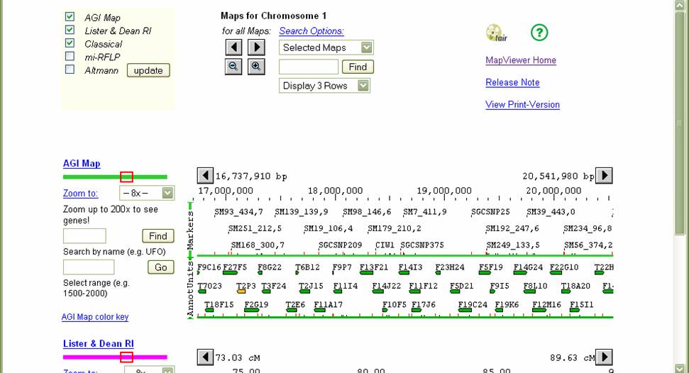
Scrolling down shows the multiple maps. AGI is a physical map in bp while Lister & Dean RI and Classical are genetic maps in Centimorgans.
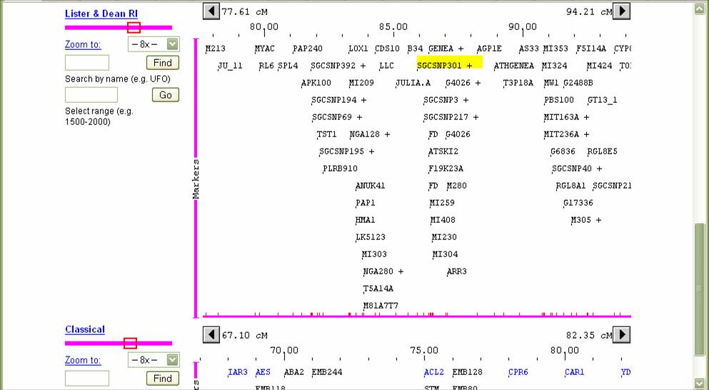
Find where the molecular markers are in the genetic map by searching for those markers on this page. If the marker appears only on the physical map, then determine its position on the AGI map by aligning the two maps by picking a close marker on the physical map and searching for that one on the genetic maps. If the search can not find that marker, you can add alternate maps (e.g. Kazusa on chromosome 3 since it may contain other markers). Double clicking on the marker itself will show more information about that marker in a new window. Aligning the different maps is important but is only an estimate- remember that the physical distance is inherently different than the genetic distance- hotspots for recombination or regions with little recombination (e.g. centromeres) can distort the relative local distances.
Once you have mapped the unknown gene to the genetic map, using recombination frequencies from the molecular markers, you can find that region by moving the genetic map (e.g. AGI) to that range in cM. You can move all maps together until you are in that range, or find that range on the genetic map search (second box on left– “select range”), and then align the physical map by searching for a common marker you see on the genetic map.
You want to then see what sequence features are in that range on the physical map.where you think the mutation lies. Note what the range of the map is on the physical map in bp. The markers present on the physical map are not all the genes- they are just markers in this region. To see what is known in this region, you need to switch to SEQUVIEWER- this shows the genome annotation of Arabidopsis. However, you now know the area of the genome in which you want to look at.
To get to SEQUVIEWER, go back to the main menu (flower TAIR icon at top right) and choose SEQUVIEW from the tools menu. You see the following screen:
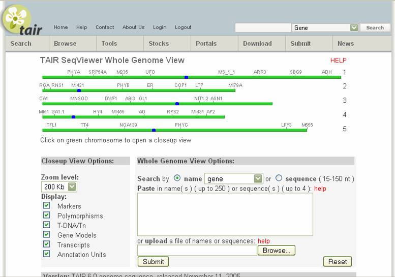
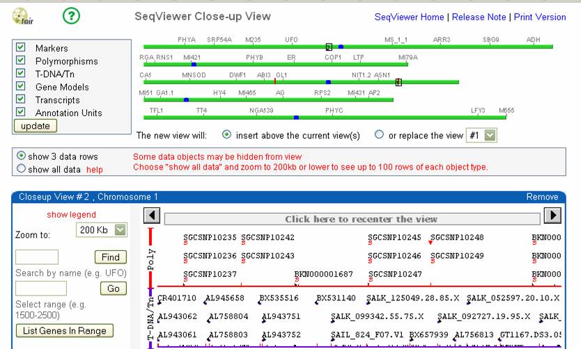
You can click on the chromosome you want and then move around on that chromosome, like in MAPVIEWER. You can also display positions of markers on this map by choosing “Marker” in the pull-down view and pasting in the marker or markers names you wish to display. This would help find a rough are to look at. For example, looking on chromosome 1:
Box shows where you are zoomed into. Markers/polymorphisms Physical map scale in bp- you
can move left or right with the arrow buttons at the top of this box, or
search for a range in bp with the second box on
the far left. Predicted Genes. Mousing over will show a summary. Double clicking will
pull up an annotation description
![]()

![]()
![]()
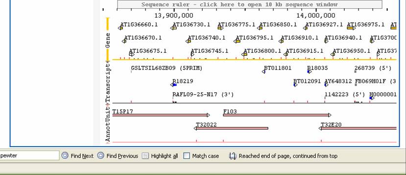
How many genes are in this area you have mapped to? What are their range of precdicted functions?. You can click on the box titled “List Genes in Range” at the left to get a list of the genes shown in the map. Note that you accumulate multiple boxes beneath this as you move around so theat one can compare multiple positions.