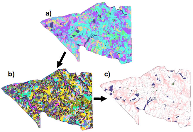
The Effective Area Model combines information about species- and context-specific edge responses with landscape maps and produces spatial grids of species-specific density predictions across a landscape. In the below graphic, the original habitat map (polygon or grid) is rendered into a new map (a) that shows each edge type and the zone closest to each edge type (b). Then, using edge responses supplied by the user (see below) for each species at each edge type, the EAM projects each species' density throughout the landscape (c). Thus, the EAM takes a patch-based realization of the landscape and converts into a continuous map of predicted habitat quality for each organism of interest. Densities are only made in habitats specified by the user (white where densities are zero, darkest pink where highest, and blue where not projected).
The EAM requires two types of data: a habitat layer and edge response parameters. The habitat layer can be a polygon file or grid, but we recommend using polygon files (see “A Note About Grids” in user's manual). Information on edge responses will be required for each species being modeled at each unique edge type within modeled habitat classes. The user must provide both the habitat layers and the edge response functions. The EAM requires parameters on edge responses for each species at each unique edge type on the landscape but only within classes specified as focal types. After specifying the attribute field that contains the habitat classes, and which specific habitat classes you wish to model (specific instructions to do this are in the user's manual), the EAM will generate a list of each unique edge type on the landscape for which parameter values are required. The user is required to enter four parameters for each of these unique edge types:
Interior_Density: This is the number of individuals per hectare that is found in the interior of the habitat (beyond the regions of edge influence, specified with Dmax). Logically, this should be the same for every edge type with the same focal habitat, but the EAM currently does not impose this restriction.
Edge_Density: This is the number of individuals per hectare that is found at the edge. This can be different for every edge type, even within the same focal habitat. Organisms may reach their edge density at the edge, or there may be a region of some width (specified with Dmin) that they maintain the same edge density.
Dmax: This specifies the distance into the habitat that all edge effects extend. Dmax can be different for each unique edge type. If Dmax is set to 0, then the model assumes no edge effects regardless of the values entered in Edge_Density or Dmin.
Dmin: This specifies the width at the edge zone over which the Edge_Density extends. For instance, if a species is never found within 100m of an edge, than the Edge_Density is 0 and Dmin is 100m.
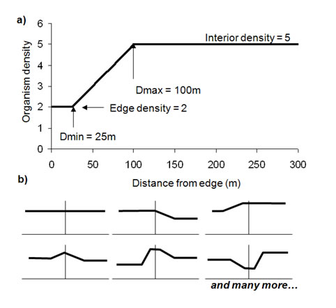
The below example (a) shows a case where organism density is lowest at the edge, and they reach there lowest density 25m from the edge and their interior density at 100m from the edge. Several different shapes can be captured with these four parameters. And since responses are specified separately on each side of the edge, then multiple shapes can be captured over the entire gradient from the interior of one habitat into the interior of the other (b).
A report showing the use of Malcolm's model in developing edge responses
Model Output:
Density grids are the main product of the EAM. As the EAM completes its run, density grids for each species are generated and automatically loaded into ArcMAP. The values in these grids can be summarized or used in several ways. The final step of the EAM dialog box allows basic summaries of the data to be generated and exported. Alternatively, users who are comfortable with ArcGIS’s rich analytical environment for grid data can perform any queries, summaries or modeling that they like. These grids could also be used as inputs for other analytical processes or programs such as Population Viability Analyses (PVAs) or Decision Support Systems (DSS) that accept raster data. Finally, these grids are useful simply for visualizing the gradation of habitat quality and could be used for mapping and demonstrations.
If the user started with a polygon map, there is an option to summarize the density grids based on any field in the attribute table of the initial map. Generally, we have used a field giving a unique identifier to each patch, but any attribute field could be chosen. There are two types of summaries the EAM will produce, one for species metrics (Species Summary) and one for landscape metrics (Edge Summary).
Summary output can be saved into .csv files, which can then be imported into any program that reads text files. The format of these files can be used for analysis. We have developed a procedure to render these files into a format that we find particularly useful for analysis. That procedure has been automated within the statistical language R in a package called “REAM”.
Download the REAM package
The EAM can be used to help guide or support management decisions, or to explore the larger-scale implications of small-scale edge effects
Demonstrations of the EAM in management
Download the EAM (includes on-line help) and installation instructions for ArcGIS 9.2 or ArcGIS 9.3
Download an example map and parameter file
View the EAM stand-alone manual